Color Matcher Pro — Guide
Step-by-step workflow and Residual (RBF) tuning guide.
Step-by-step workflow and Residual (RBF) tuning guide.
This example matches Fujifilm Provia (Ref A) to Fujifilm film simulation Classic Negative (Ref B). The Ref B files use the ClassigNeg_X-T5*.avif naming.
Ref A (Fujifilm Provia)
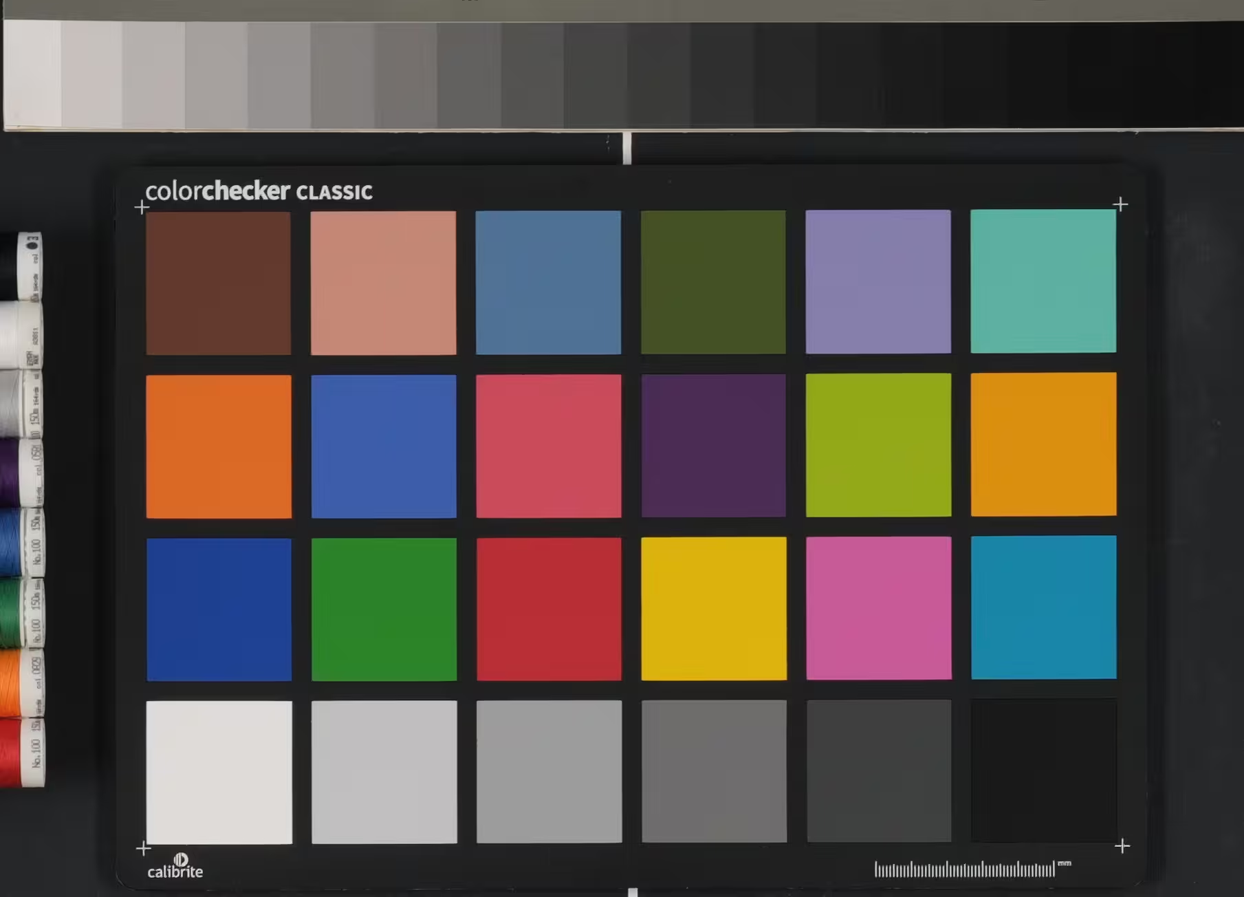
Base reference: PROVIA_X-T5_0.avif
Ref B (Fujifilm Classic Negative)
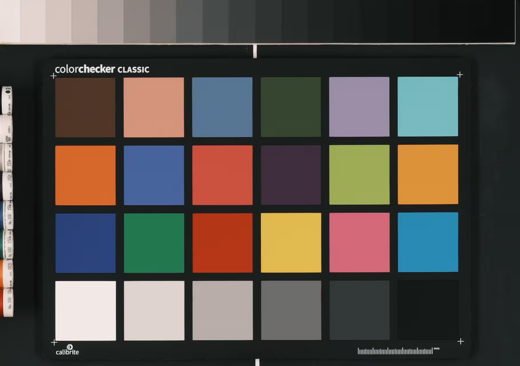
Base reference: ClassigNeg_X-T5_0.avif
Suggested flow: load PROVIA_X-T5_0.avif and ClassigNeg_X-T5_0.avif, sample gray then color patches, run Calculate Base, and only then extract Residuals if the match still looks too clean or misses hue shifts typical of Classic Negative. If residuals are too strong, reduce Strength to 70-85% and increase Sigma slightly.
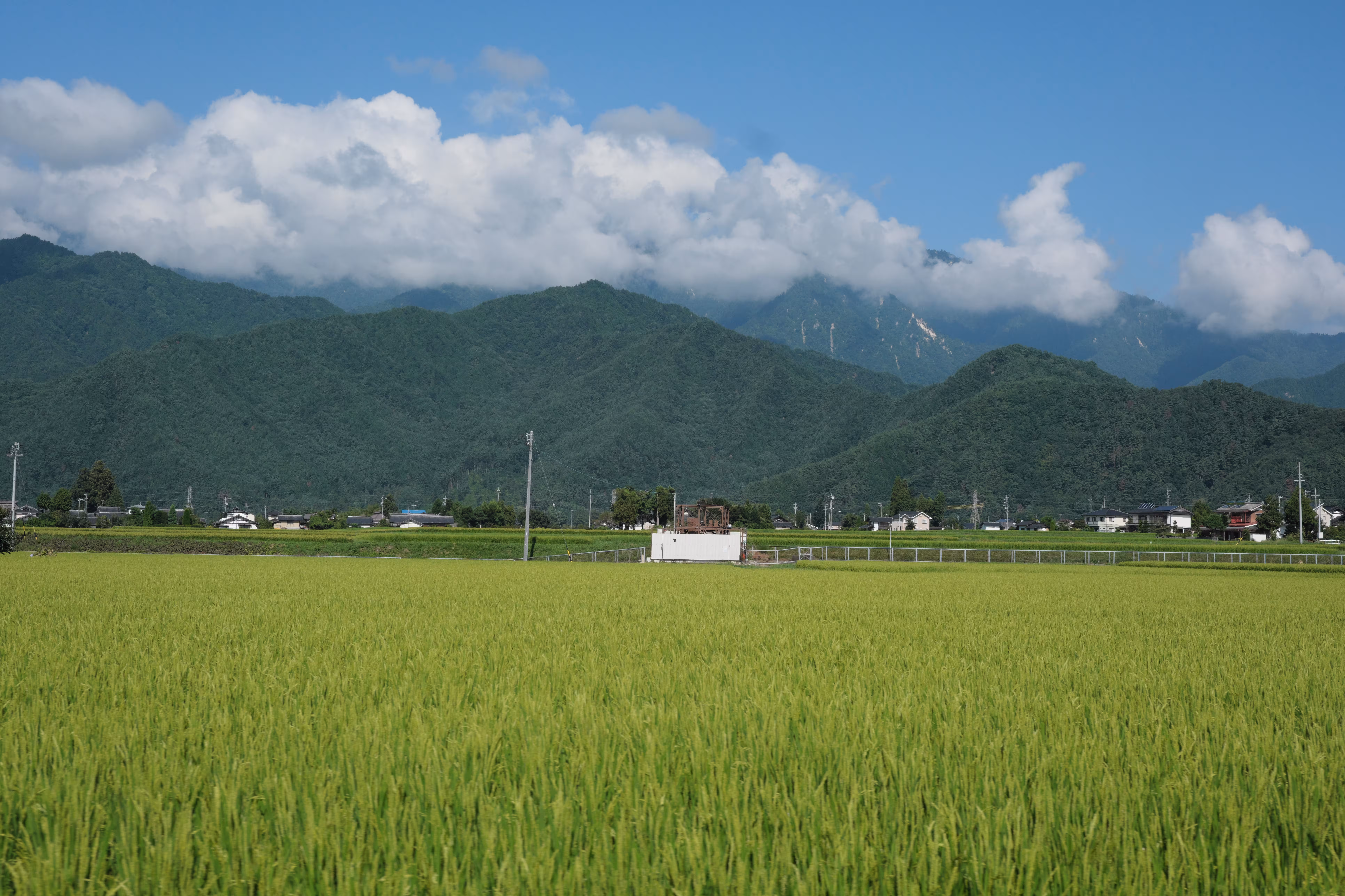
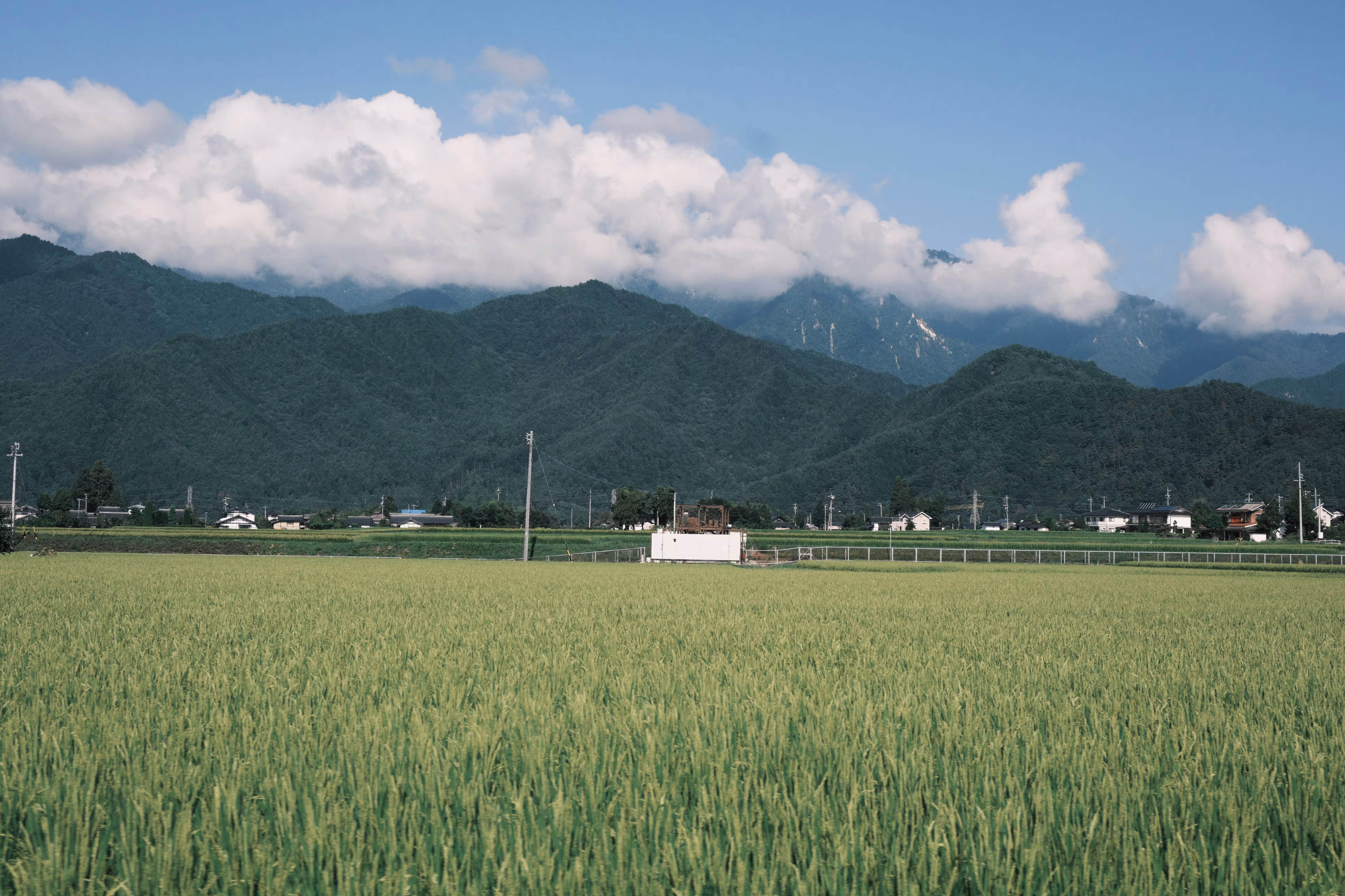
The following images show the original photo, the official Classic Negative conversion from Fujifilm Raw Converter, and the Color Matcher result.
Original → Result (Diff)
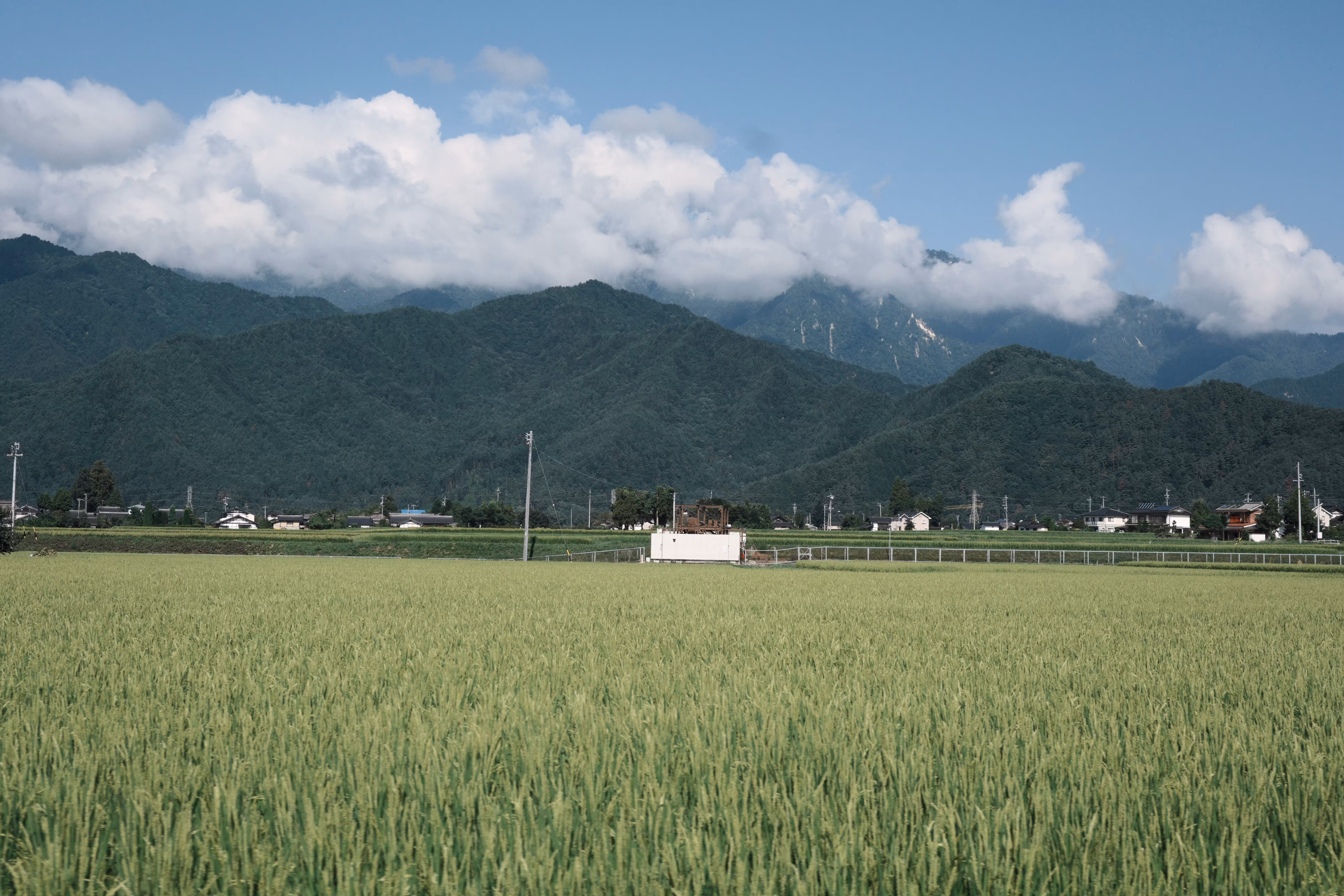
Classic Negative (Fujifilm RAW Converter)
_DSF6321_CLASSICNEG.avif
For a quick overview of the tool UI, see the following screenshot.
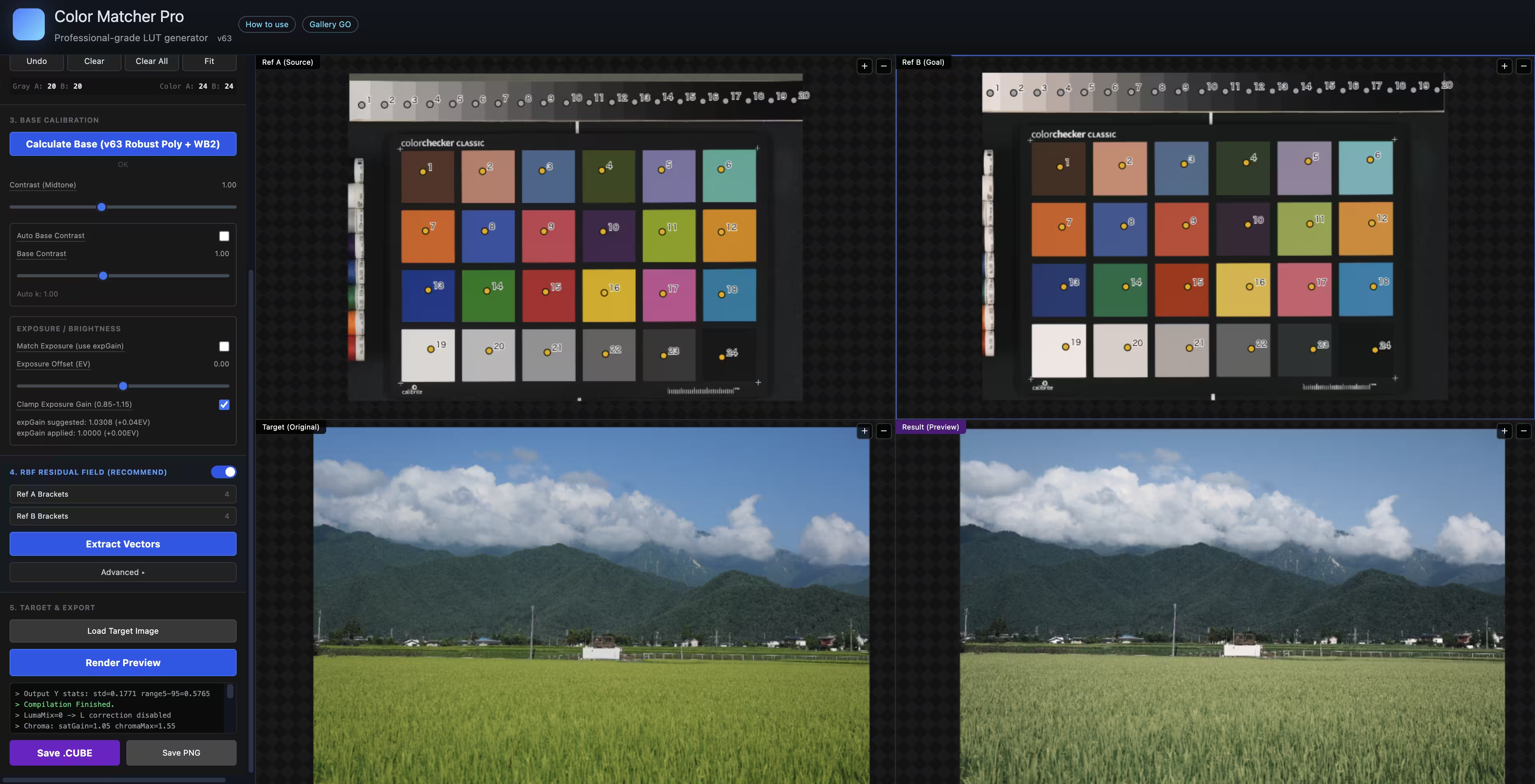
This page summarizes the core workflow and provides a more detailed explanation of the Residual (RBF) stage. For parameter-by-parameter guidance, refer to the tool UI tooltips.
1. Load reference images — Load Ref A (Source) and Ref B (Goal). Similar exposure and white balance will produce more stable matching and reduce outliers.
2. Sample patches — Collect Gray first, then Color. Auto Grid is ideal for standard charts; Manual is better for irregular or partial charts.
3. Calculate Base — Run Calculate Base to build the main transform. After this completes, you can preview and extract residuals.
4. Residual + Export — Use Residuals to correct subtle color errors that the Base matrix cannot capture. After extracting residuals, render a preview and export the .CUBE.
As a practical reference, see DPReview. The idea is to photograph a color chart and a grayscale chart, then develop RAW files at multiple exposures to create bracketed sets. This produces consistent patch samples across a wider dynamic range, which improves residual extraction stability.
Residuals are learned as correction vectors in OKLab space. For each sampled patch, the tool compares the Base-predicted color to the target color and stores the delta as a small vector. These vectors are clustered on a 3D OKLab grid to reduce noise, then interpolated with a radial basis function (RBF) when generating the LUT. This lets the model preserve the global look from Base while fixing localized hue or saturation drift.